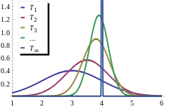
Consistent estimator

For broader coverage of this topic, see Consistency (statistics).

{T₁, T₂, T₃, ...} is a sequence of estimators for parameter θ₀, the true value of which is 4. This sequence is consistent: the estimators are getting more and more concentrated near the true value θ₀; at the same time, these estimators are biased. The limiting distribution of the sequence is a degenerate random variable which equals θ₀ with probability 1.

In statistics, a consistent estimator or asymptotically consistent estimator is an estimator—a rule for computing estimates of a parameter θ₀—having the property that as the number of data points used increases indefinitely, the resulting sequence of estimates converges in probability to θ₀. This means that the distributions of the estimates become more and more concentrated near the true value of the parameter being estimated, so that the probability of the estimator being arbitrarily close to θ₀ converges to one.

In practice one constructs an estimator as a function of an available sample of size n, and then imagines being able to keep collecting data and expanding the sample ad infinitum. In this way one would obtain a sequence of estimates indexed by n, and consistency is a property of what occurs as the sample size “grows to infinity”. If the sequence of estimates can be mathematically shown to converge in probability to the true value θ₀, it is called a consistent estimator; otherwise the estimator is said to be inconsistent.

Consistency as defined here is sometimes referred to as weak consistency. When we replace convergence in probability with almost sure convergence, then the estimator is said to be strongly consistent. Consistency is related to bias; see bias versus consistency.

Definition

Formally speaking, an estimator T_n of parameter θ is said to be weakly consistent, if it converges in probability to the true value of the parameter:[1]

${\displaystyle {\underset {n\to \infty }{\operatorname {plim} }}\;T_{n}=\theta .}$

i.e. if, for all ε > 0

${\displaystyle \lim _{n\to \infty }\Pr {\big (}|T_{n}-\theta |>\varepsilon {\big )}=0.}$

An estimator T_n of parameter θ is said to be strongly consistent, if it converges almost surely to the true value of the parameter:

${\displaystyle \Pr {\big (}\lim _{n\to \infty }T_{n}=\theta {\big )}=1.}$

A more rigorous definition takes into account the fact that θ is actually unknown, and thus, the convergence in probability must take place for every possible value of this parameter. Suppose {p_θ: θ ∈ Θ} is a family of distributions (the parametric model), and X^θ = {X₁, X₂, … : X_i ~ p_θ} is an infinite sample from the distribution p_θ. Let { T_n(X^θ) } be a sequence of estimators for some parameter g(θ). Usually, T_n will be based on the first n observations of a sample. Then this sequence {T_n} is said to be (weakly) consistent if [2]

${\displaystyle {\underset {n\to \infty }{\operatorname {plim} }}\;T_{n}(X^{\theta })=g(\theta ),\ \ {\text{for all}}\ \theta \in \Theta .}$

This definition uses g(θ) instead of simply θ, because often one is interested in estimating a certain function or a sub-vector of the underlying parameter. In the next example, we estimate the location parameter of the model, but not the scale:

Examples

Sample mean of a normal random variable

Suppose one has a sequence of statistically independent observations {X₁, X₂, ...} from a normal N(μ, σ^2) distribution. To estimate μ based on the first n observations, one can use the sample mean: T_n = (X₁ + ... + X_n)/n. This defines a sequence of estimators, indexed by the sample size n.

From the properties of the normal distribution, we know the sampling distribution of this statistic: T_n is itself normally distributed, with mean μ and variance σ^2/n. Equivalently, ${\displaystyle \scriptstyle (T_{n}-\mu )/(\sigma /{\sqrt {n}})}$ has a standard normal distribution:

${\displaystyle \Pr \!\left[\,|T_{n}-\mu |\geq \varepsilon \,\right]=\Pr \!\left[{\frac {{\sqrt {n}}\,{\big |}T_{n}-\mu {\big |}}{\sigma }}\geq {\sqrt {n}}\varepsilon /\sigma \right]=2\left(1-\Phi \left({\frac {{\sqrt {n}}\,\varepsilon }{\sigma }}\right)\right)\to 0}$

as n tends to infinity, for any fixed ε > 0. Therefore, the sequence T_n of sample means is consistent for the population mean μ (recalling that ${\displaystyle \Phi }$ is the cumulative distribution of the normal distribution).

Establishing consistency

The notion of asymptotic consistency is very close, almost synonymous to the notion of convergence in probability. As such, any theorem, lemma, or property which establishes convergence in probability may be used to prove the consistency. Many such tools exist:

• In order to demonstrate consistency directly from the definition one can use the inequality [3]

${\displaystyle \Pr \!{\big [}h(T_{n}-\theta )\geq \varepsilon {\big ]}\leq {\frac {\operatorname {E} {\big [}h(T_{n}-\theta ){\big ]}}{h(\varepsilon )}},}$

the most common choice for function h being either the absolute value (in which case it is known as Markov inequality), or the quadratic function (respectively Chebyshev's inequality).

• Another useful result is the continuous mapping theorem: if T_n is consistent for θ and g(·) is a real-valued function continuous at point θ, then g(T_n) will be consistent for g(θ):[4]

${\displaystyle T_{n}\ {\xrightarrow {p}}\ \theta \ \quad \Rightarrow \quad g(T_{n})\ {\xrightarrow {p}}\ g(\theta )}$

• Slutsky's theorem can be used to combine several different estimators, or an estimator with a non-random convergent sequence. If T_n →^dα, and S_n →^pβ, then [5]

${\displaystyle {\begin{aligned}&T_{n}+S_{n}\ {\xrightarrow {d}}\ \alpha +\beta ,\\&T_{n}S_{n}\ {\xrightarrow {d}}\ \alpha \beta ,\\&T_{n}/S_{n}\ {\xrightarrow {d}}\ \alpha /\beta ,{\text{ provided that }}\beta \neq 0\end{aligned}}}$

• If estimator T_n is given by an explicit formula, then most likely the formula will employ sums of random variables, and then the law of large numbers can be used: for a sequence {X_n} of random variables and under suitable conditions,

${\displaystyle {\frac {1}{n}}\sum _{i=1}^{n}g(X_{i})\ {\xrightarrow {p}}\ \operatorname {E} [\,g(X)\,]}$

• If estimator T_n is defined implicitly, for example as a value that maximizes certain objective function (see extremum estimator), then a more complicated argument involving stochastic equicontinuity has to be used.[6]

Bias versus consistency

Unbiased but not consistent

An estimator can be unbiased but not consistent. For example, for an iid sample {x
₁,..., x
_n} one can use T
_n(X) = x
_n as the estimator of the mean E[X]. Note that here the sampling distribution of T
_n is the same as the underlying distribution (for any n, as it ignores all points but the last), so E[T
_n(X)] = E[X] and it is unbiased, but it does not converge to any value.

However, if a sequence of estimators is unbiased and converges to a value, then it is consistent, as it must converge to the correct value.

Biased but consistent

Alternatively, an estimator can be biased but consistent. For example, if the mean is estimated by ${\displaystyle {1 \over n}\sum x_{i}+{1 \over n}}$ it is biased, but as ${\displaystyle n\rightarrow \infty }$, it approaches the correct value, and so it is consistent.

Important examples include the sample variance and sample standard deviation. Without Bessel's correction (that is, when using the sample size ${\displaystyle n}$ instead of the degrees of freedom ${\displaystyle n-1}$), these are both negatively biased but consistent estimators. With the correction, the corrected sample variance is unbiased, while the corrected sample standard deviation is still biased, but less so, and both are still consistent: the correction factor converges to 1 as sample size grows.

Here is another example. Let ${\displaystyle T_{n}}$ be a sequence of estimators for ${\displaystyle \theta }$.

${\displaystyle \Pr(T_{n})={\begin{cases}1-1/n,&{\mbox{if }}\,T_{n}=\theta \\1/n,&{\mbox{if }}\,T_{n}=n\delta +\theta \end{cases}}}$

We can see that ${\displaystyle T_{n}{\xrightarrow {p}}\theta }$, ${\displaystyle \operatorname {E} [T_{n}]=\theta +\delta }$, and the bias does not converge to zero.

See also

• Efficient estimator
• Fisher consistency — alternative, although rarely used concept of consistency for the estimators
• Regression dilution
• Statistical hypothesis testing
• Instrumental variables estimation

Notes

1. Amemiya 1985, Definition 3.4.2.
2. Lehman & Casella 1998, p. 332.
3. Amemiya 1985, equation (3.2.5).
4. Amemiya 1985, Theorem 3.2.6.
5. Amemiya 1985, Theorem 3.2.7.
6. Newey & McFadden 1994, Chapter 2.

References

• Amemiya, Takeshi (1985). Advanced Econometrics. Harvard University Press. ISBN 0-674-00560-0.
• Lehmann, E. L.; Casella, G. (1998). Theory of Point Estimation (2nd ed.). Springer. ISBN 0-387-98502-6.
• Newey, W. K.; McFadden, D. (1994). "Chapter 36: Large sample estimation and hypothesis testing". In Robert F. Engle; Daniel L. McFadden (eds.). Handbook of Econometrics. Vol. 4. Elsevier Science. ISBN 0-444-88766-0. S2CID 29436457.
• Nikulin, M. S. (2001) [1994], "Consistent estimator", Encyclopedia of Mathematics, EMS Press
• Sober, E. (1988), "Likelihood and convergence", Philosophy of Science, 55 (2): 228–237, doi:10.1086/289429.

External links

• Econometrics lecture (topic: unbiased vs. consistent) on YouTube by Mark Thoma