|
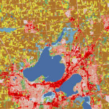
Spatial heterogeneity Spatial heterogeneity is a property generally ascribed to a landscape or to a population. It refers to the uneven distribution of various concentrations of each species within an area. A landscape with spatial heterogeneity has a mix of concentrations of multiple species of plants or animals (biological), or of terrain formations (geological), or environmental characteristics (e.g. rainfall, temperature, wind) filling its area. A population showing spatial heterogeneity is one where various concentrations of individuals of this species are unevenly distributed across an area; nearly synonymous with "patchily distributed." TerminologySpatial heterogeneity can be re-phrased as scaling hierarchy of far more small things than large ones. It has been formulated as a scaling law.[1] Spatial heterogeneity or scaling hierarchy can be measured or quantified by ht-index: a head/tail breaks induced number. [2][3] ExamplesEnvironments with a wide variety of habitats such as different topographies, soil types, and climates are able to accommodate a greater amount of species. The leading scientific explanation for this is that when organisms can finely subdivide a landscape into unique suitable habitats, more species can coexist in a landscape without competition, a phenomenon termed "niche partitioning." Spatial heterogeneity is a concept parallel to ecosystem productivity, the species richness of animals is directly related to the species richness of plants in a certain habitat. Vegetation serves as food sources, habitats, and so on. Therefore, if vegetation is scarce, the animal populations will be as well. The more plant species there are in an ecosystem, the greater variety of microhabitats there are. Plant species richness directly reflects spatial heterogeneity in an ecosystem. TypesThere exist two main types of spatial heterogeneity. The spatial local heterogeneity categorises the geographic phenomena whose its attributes' values are significantly similar within a directly local neighbourhood, but which significantly differ in the nearby surrounding-areas beyond this directly local neighbourhood (e.g. hot spots, cold spots). The spatial stratified heterogeneity categorises the geographic phenomena whose the within-strata variance of its attributes' values is significantly lower than its between-strata variance, such as collections of ecological zones or land-use classes within a given geographic area depict.[4] TestingSpatial local heterogeneity can be tested by LISA, Gi and SatScan, while spatial stratified heterogeneity of an attribute can be measured by geographical detector q-statistic:[4] where a population is partitioned into h = 1, ..., L strata; N stands for the size of the population, σ2 stands for variance of the attribute. The value of q is within [0, 1], 0 indicates no spatial stratified heterogeneity, 1 indicates perfect spatial stratified heterogeneity. The value of q indicates the percent of the variance of an attribute explained by the stratification. The q follows a noncentral F probability density function.  Spatial heterogeneity for multivariate data and 3D data can also be statistically assessed using the "HTA index (HeTerogeneity Average index)".:[5]  ModelsSpatial stratified heterogeneityOptimal parameters-based geographical detectorOptimal Parameters-based Geographical Detector (OPGD) characterizes spatial heterogeneity with the optimized parameters of spatial data discretization for identifying geographical factors and interactive impacts of factors, and estimating risks.[6][7] Interactive detector for spatial associationsInteractive Detector for Spatial Associations (IDSA) estimates power of interactive determinants (PID) on the basis of spatial stratified heterogeneity, spatial autocorrelation, and spatial fuzzy overlay of explanatory variables.[8] Geographically optimal zones-based heterogeneityGeographically Optimal Zones-based Heterogeneity (GOZH) explores individual and interactive determinants of geographical attributes (e.g., global soil moisture) across a large study area based on the identification of explainable geographically optimal zones.[9] Robust geographical detectorRobust Geographical Detector (RGD) overcomes the limitation of the sensitivity in spatial data discretization and estimates robust power of determinants of explanatory variables.[10] meta-STARThe model-agnostic Spatial Transformation And modeRation (meta-STAR) is a framework for integrating the spatial heterogeneity into spatial statistical models (e.g. spatial ensemble methods, spatial neural networks), so to improve their accuracy. It involves the use of spatial networks/transformations and spatial moderators, plus handles the geo-spatial datasets representing geographic phenomena at multiple scales.[11] Law of geographyIn a 2004 publication titled "The Validity and Usefulness of Laws in Geographic Information Science and Geography," Michael Frank Goodchild proposed Spatial heterogeneity could be a candidate for a law of geography similar to Tobler's first law of geography.[12] The literature cites this paper and states this law as "geographic variables exhibit uncontrolled variance."[12][13][14] Often referred to as the second law of geography, or Michael Goodchild's second law of geography, it is one of many concepts competing for that term, including Tobler's second law of geography, and Arbia's law of geography.[13][14][15] See alsoReferences
|
