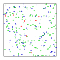
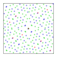
Quasi-Monte Carlo method

Pseudorandom sequence

A Sobol sequence of low-discrepancy quasi-random numbers, showing the first 10 (red), 100 (red+blue) and 256 (red+blue+green) points from the sequence.

256 points from a pseudorandom number source, and Sobol sequence (red=1,..,10, blue=11,..,100, green=101,..,256). Points from Sobol sequence are more evenly distributed.

In numerical analysis, the quasi-Monte Carlo method is a method for numerical integration and solving some other problems using low-discrepancy sequences (also called quasi-random sequences or sub-random sequences) to achieve variance reduction. This is in contrast to the regular Monte Carlo method or Monte Carlo integration, which are based on sequences of pseudorandom numbers.

Monte Carlo and quasi-Monte Carlo methods are stated in a similar way. The problem is to approximate the integral of a function f as the average of the function evaluated at a set of points x₁, ..., x_N:

${\displaystyle \int _{[0,1]^{s}}f(u)\,{\rm {d}}u\approx {\frac {1}{N}}\,\sum _{i=1}^{N}f(x_{i}).}$

Since we are integrating over the s-dimensional unit cube, each x_i is a vector of s elements. The difference between quasi-Monte Carlo and Monte Carlo is the way the x_i are chosen. Quasi-Monte Carlo uses a low-discrepancy sequence such as the Halton sequence, the Sobol sequence, or the Faure sequence, whereas Monte Carlo uses a pseudorandom sequence. The advantage of using low-discrepancy sequences is a faster rate of convergence. Quasi-Monte Carlo has a rate of convergence close to O(1/N), whereas the rate for the Monte Carlo method is O(N^−0.5).[1]

The Quasi-Monte Carlo method recently became popular in the area of mathematical finance or computational finance.[1] In these areas, high-dimensional numerical integrals, where the integral should be evaluated within a threshold ε, occur frequently. Hence, the Monte Carlo method and the quasi-Monte Carlo method are beneficial in these situations.

Approximation error bounds of quasi-Monte Carlo

The approximation error of the quasi-Monte Carlo method is bounded by a term proportional to the discrepancy of the set x₁, ..., x_N. Specifically, the Koksma–Hlawka inequality states that the error

${\displaystyle \varepsilon =\left|\int _{[0,1]^{s}}f(u)\,{\rm {d}}u-{\frac {1}{N}}\,\sum _{i=1}^{N}f(x_{i})\right|}$

is bounded by

${\displaystyle |\varepsilon |\leq V(f)D_{N},}$

where V(f) is the Hardy–Krause variation of the function f (see Morokoff and Caflisch (1995) [2] for the detailed definitions). D_N is the so-called star discrepancy of the set (x₁,...,x_N) and is defined as

${\displaystyle D_{N}=\sup _{Q\subset [0,1]^{s}}\left|{\frac {{\text{number of points in }}Q}{N}}-\operatorname {volume} (Q)\right|,}$

where Q is a rectangular solid in [0,1]^s with sides parallel to the coordinate axes.[2] The inequality ${\displaystyle |\varepsilon |\leq V(f)D_{N}}$ can be used to show that the error of the approximation by the quasi-Monte Carlo method is ${\displaystyle O\left({\frac {(\log N)^{s}}{N}}\right)}$, whereas the Monte Carlo method has a probabilistic error of ${\displaystyle O\left({\frac {1}{\sqrt {N}}}\right)}$. Thus, for sufficiently large ${\displaystyle N}$, quasi-Monte Carlo will always outperform random Monte Carlo. However, ${\displaystyle \log(N)^{s}}$ grows exponentially quickly with the dimension, meaning a poorly-chosen sequence can be much worse than Monte Carlo in high dimensions. In practice, it is almost always possible to select an appropriate low-discrepancy sequence, or apply an appropriate transformation to the integrand, to ensure that quasi-Monte Carlo performs at least as well as Monte Carlo (and often much better).[1]

Monte Carlo and quasi-Monte Carlo for multidimensional integrations

For one-dimensional integration, quadrature methods such as the trapezoidal rule, Simpson's rule, or Newton–Cotes formulas are known to be efficient if the function is smooth. These approaches can be also used for multidimensional integrations by repeating the one-dimensional integrals over multiple dimensions. However, the number of function evaluations grows exponentially as s, the number of dimensions, increases. Hence, a method that can overcome this curse of dimensionality should be used for multidimensional integrations. The standard Monte Carlo method is frequently used when the quadrature methods are difficult or expensive to implement.[2] Monte Carlo and quasi-Monte Carlo methods are accurate and relatively fast when the dimension is high, up to 300 or higher.[3]

Morokoff and Caflisch [2] studied the performance of Monte Carlo and quasi-Monte Carlo methods for integration. In the paper, Halton, Sobol, and Faure sequences for quasi-Monte Carlo are compared with the standard Monte Carlo method using pseudorandom sequences. They found that the Halton sequence performs best for dimensions up to around 6; the Sobol sequence performs best for higher dimensions; and the Faure sequence, while outperformed by the other two, still performs better than a pseudorandom sequence.

However, Morokoff and Caflisch [2] gave examples where the advantage of the quasi-Monte Carlo is less than expected theoretically. Still, in the examples studied by Morokoff and Caflisch, the quasi-Monte Carlo method did yield a more accurate result than the Monte Carlo method with the same number of points. Morokoff and Caflisch remark that the advantage of the quasi-Monte Carlo method is greater if the integrand is smooth, and the number of dimensions s of the integral is small.

Drawbacks of quasi-Monte Carlo

Lemieux mentioned the drawbacks of quasi-Monte Carlo:[4]

• In order for ${\displaystyle O\left({\frac {(\log N)^{s}}{N}}\right)}$ to be smaller than ${\displaystyle O\left({\frac {1}{\sqrt {N}}}\right)}$, ${\displaystyle s}$ needs to be small and ${\displaystyle N}$ needs to be large (e.g. ${\displaystyle N>2^{s}}$). For large s, depending on the value of N, the discrepancy of a point set from a low-discrepancy generator might be not smaller than for a random set.
• For many functions arising in practice, ${\displaystyle V(f)=\infty }$ (e.g. if Gaussian variables are used).
• We only know an upper bound on the error (i.e., ε ≤ V(f) D_N) and it is difficult to compute ${\displaystyle D_{N}^{*}}$ and ${\displaystyle V(f)}$.

In order to overcome some of these difficulties, we can use a randomized quasi-Monte Carlo method.

Randomization of quasi-Monte Carlo

Since the low discrepancy sequence are not random, but deterministic, quasi-Monte Carlo method can be seen as a deterministic algorithm or derandomized algorithm. In this case, we only have the bound (e.g., ε ≤ V(f) D_N) for error, and the error is hard to estimate. In order to recover our ability to analyze and estimate the variance, we can randomize the method (see randomization for the general idea). The resulting method is called the randomized quasi-Monte Carlo method and can be also viewed as a variance reduction technique for the standard Monte Carlo method.[5] Among several methods, the simplest transformation procedure is through random shifting. Let {x₁,...,x_N} be the point set from the low discrepancy sequence. We sample s-dimensional random vector U and mix it with {x₁, ..., x_N}. In detail, for each x_j, create

${\displaystyle y_{j}=x_{j}+U{\pmod {1}}}$

and use the sequence ${\displaystyle (y_{j})}$ instead of ${\displaystyle (x_{j})}$. If we have R replications for Monte Carlo, sample s-dimensional random vector U for each replication. Randomization allows to give an estimate of the variance while still using quasi-random sequences. Compared to pure quasi Monte-Carlo, the number of samples of the quasi random sequence will be divided by R for an equivalent computational cost, which reduces the theoretical convergence rate. Compared to standard Monte-Carlo, the variance and the computation speed are slightly better from the experimental results in Tuffin (2008) [6]

See also

• Monte Carlo method – Probabilistic problem-solving algorithm
• Monte Carlo methods in finance – Probabilistic measurement methods
• Quasi-Monte Carlo methods in finance
• Biology Monte Carlo method – Method for simulating ion transport
• Computational physics – Numerical simulations of physical problems via computers
• Low-discrepancy sequences – Type of mathematical sequencePages displaying short descriptions of redirect targets
• Discrepancy theory – Theory of irregularities of distribution
• Markov chain Monte Carlo – Calculation of complex statistical distributions

References

1. Søren Asmussen and Peter W. Glynn, Stochastic Simulation: Algorithms and Analysis, Springer, 2007, 476 pages
2. William J. Morokoff and Russel E. Caflisch, Quasi-Monte Carlo integration, J. Comput. Phys. 122 (1995), no. 2, 218–230. (At CiteSeer: [1])
3. Rudolf Schürer, A comparison between (quasi-)Monte Carlo and cubature rule based methods for solving high-dimensional integration problems, Mathematics and Computers in Simulation, Volume 62, Issues 3–6, 3 March 2003, 509–517
4. Christiane Lemieux, Monte Carlo and Quasi-Monte Carlo Sampling, Springer, 2009, ISBN 978-1441926760
5. Moshe Dror, Pierre L’Ecuyer and Ferenc Szidarovszky, Modeling Uncertainty: An Examination of Stochastic Theory, Methods, and Applications, Springer 2002, pp. 419-474
6. Bruno Tuffin, Randomization of Quasi-Monte Carlo Methods for Error Estimation: Survey and Normal Approximation, Monte Carlo Methods and Applications mcma. Volume 10, Issue 3-4, Pages 617–628, ISSN (Online) 1569-3961, ISSN (Print) 0929-9629, doi:10.1515/mcma.2004.10.3-4.617, May 2008

• R. E. Caflisch, Monte Carlo and quasi-Monte Carlo methods, Acta Numerica vol. 7, Cambridge University Press, 1998, pp. 1–49.
• Josef Dick and Friedrich Pillichshammer, Digital Nets and Sequences. Discrepancy Theory and Quasi-Monte Carlo Integration, Cambridge University Press, Cambridge, 2010, ISBN 978-0-521-19159-3
• Gunther Leobacher and Friedrich Pillichshammer, Introduction to quasi-Monte Carlo Integration and Applications, Compact Textbooks in Mathematics, Birkhäuser, 2014, ISBN 978-3-319-03424-9
• Michael Drmota and Robert F. Tichy, Sequences, discrepancies and applications, Lecture Notes in Math., 1651, Springer, Berlin, 1997, ISBN 3-540-62606-9
• William J. Morokoff and Russel E. Caflisch, Quasi-random sequences and their discrepancies, SIAM J. Sci. Comput. 15 (1994), no. 6, 1251–1279 (At CiteSeer:[2])
• Harald Niederreiter. Random Number Generation and Quasi-Monte Carlo Methods. Society for Industrial and Applied Mathematics, 1992. ISBN 0-89871-295-5
• Harald G. Niederreiter, Quasi-Monte Carlo methods and pseudo-random numbers, Bull. Amer. Math. Soc. 84 (1978), no. 6, 957–1041
• Oto Strauch and Štefan Porubský, Distribution of Sequences: A Sampler, Peter Lang Publishing House, Frankfurt am Main 2005, ISBN 3-631-54013-2

External links

• The MCQMC Wiki page contains a lot of free online material on Monte Carlo and quasi-Monte Carlo methods
• A very intuitive and comprehensive introduction to Quasi-Monte Carlo methods