|
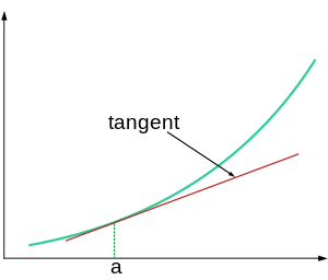
Linear approximation In mathematics, a linear approximation is an approximation of a general function using a linear function (more precisely, an affine function). They are widely used in the method of finite differences to produce first order methods for solving or approximating solutions to equations. DefinitionGiven a twice continuously differentiable function of one real variable, Taylor's theorem for the case states that where is the remainder term. The linear approximation is obtained by dropping the remainder: This is a good approximation when is close enough to ; since a curve, when closely observed, will begin to resemble a straight line. Therefore, the expression on the right-hand side is just the equation for the tangent line to the graph of at . For this reason, this process is also called the tangent line approximation. Linear approximations in this case are further improved when the second derivative of a, , is sufficiently small (close to zero) (i.e., at or near an inflection point). If is concave down in the interval between and , the approximation will be an overestimate (since the derivative is decreasing in that interval). If is concave up, the approximation will be an underestimate.[1] Linear approximations for vector functions of a vector variable are obtained in the same way, with the derivative at a point replaced by the Jacobian matrix. For example, given a differentiable function with real values, one can approximate for close to by the formula The right-hand side is the equation of the plane tangent to the graph of at In the more general case of Banach spaces, one has where is the Fréchet derivative of at . ApplicationsOpticsGaussian optics is a technique in geometrical optics that describes the behaviour of light rays in optical systems by using the paraxial approximation, in which only rays which make small angles with the optical axis of the system are considered.[2] In this approximation, trigonometric functions can be expressed as linear functions of the angles. Gaussian optics applies to systems in which all the optical surfaces are either flat or are portions of a sphere. In this case, simple explicit formulae can be given for parameters of an imaging system such as focal distance, magnification and brightness, in terms of the geometrical shapes and material properties of the constituent elements. Period of oscillationThe period of swing of a simple gravity pendulum depends on its length, the local strength of gravity, and to a small extent on the maximum angle that the pendulum swings away from vertical, θ0, called the amplitude.[3] It is independent of the mass of the bob. The true period T of a simple pendulum, the time taken for a complete cycle of an ideal simple gravity pendulum, can be written in several different forms (see pendulum), one example being the infinite series:[4][5] where L is the length of the pendulum and g is the local acceleration of gravity. However, if one takes the linear approximation (i.e. if the amplitude is limited to small swings,[Note 1] ) the period is:[6]
In the linear approximation, the period of swing is approximately the same for different size swings: that is, the period is independent of amplitude. This property, called isochronism, is the reason pendulums are so useful for timekeeping.[7] Successive swings of the pendulum, even if changing in amplitude, take the same amount of time. Electrical resistivityThe electrical resistivity of most materials changes with temperature. If the temperature T does not vary too much, a linear approximation is typically used: where is called the temperature coefficient of resistivity, is a fixed reference temperature (usually room temperature), and is the resistivity at temperature . The parameter is an empirical parameter fitted from measurement data. Because the linear approximation is only an approximation, is different for different reference temperatures. For this reason it is usual to specify the temperature that was measured at with a suffix, such as , and the relationship only holds in a range of temperatures around the reference.[8] When the temperature varies over a large temperature range, the linear approximation is inadequate and a more detailed analysis and understanding should be used. See also
Notes
References
Further reading
|


![{\displaystyle \rho (T)=\rho _{0}[1+\alpha (T-T_{0})]}](https://wikimedia.org/api/rest_v1/media/math/render/svg/7f0d28efd73ce74b1399b50c01300a171066e9be)


